Calculating shap values can take an extremely long time. fastshap was designed to be as fast as possible by utilizing inner and outer batch assignments to keep the calculations inside vectorized operations as often as it can. This includes the model evaluation. If the model in question is more efficient for 100 samples than 10, then this sort of vectorization can have enormous benefits.

This package specifically offers a kernel explainer. Kernel explainers can calculate approximate shap values of f(X) towards y for any function f. Much faster shap solutions are available specifically for gradient boosted trees and deep neural networks.

A kernel explainer is ideal in situations where:

1. The model you are using does not have model-specific methods available (for example, support vector machine)
2. You need to explain a modeling pipeline which includes variable transformations.
3. The model has a link function or some other target transformation. For example, you wish to explain the raw probabilities in a classification model, instead of the log-odds.

Advantages of fastshap:

• Fast. See benchmarks for comparisons.
• Native handling of both numpy arrays and pandas dataframes including principled treatment of categories.
• Easy built in stratification of background set.
• Capable of plotting categorical variables in dependence plots.
• Capable of determining categorical variable interactions in shap values.
• Capable of plotting missing values in interaction variable.

Disadvantages of fastshap:

• Only dependency plotting is supported as of now.
• Does not support feature groups yet.
• Does not support weights yet.

This package can be installed using pip:

# Using pip
$ pip install fastshap --no-cache-dir

You can also download the latest development version from this repository. If you want to install from github with conda, you must first run conda install pip git.

$ pip install git+https://github.com/AnotherSamWilson/fastshap.git

These benchmarks compare the shap package KernelExplainer to the one in fastshap. All code is in ./benchmarks. We left out model-specific shap explainers, because they are usually orders of magnitued faster and more efficient than kernel explainers.

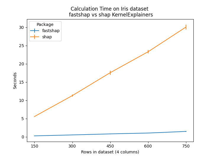
The iris dataset is a table of 150 rows and 5 columns (4 features, one target). This benchmark measured the time to calculate the shap values for different row counts. The iris dataset was concatenated to itself to get the desired dataset size:

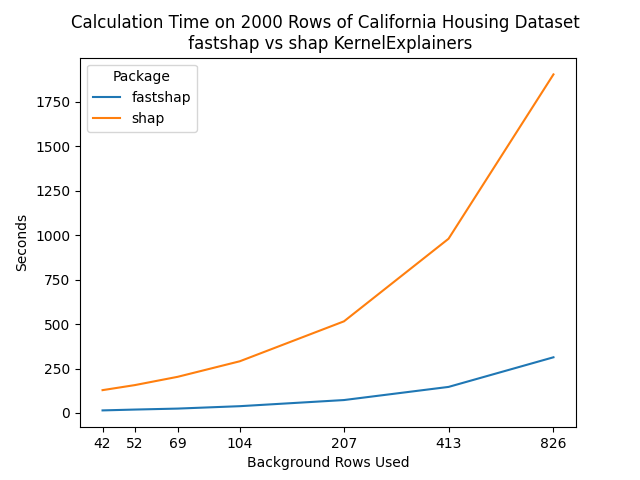
The California Housing dataset is a table of 20640 rows and 9 columns (8 features, one target). This benchmark measured the time it took to calculate shap values on the first 2000 rows for different sizes of the background dataset.

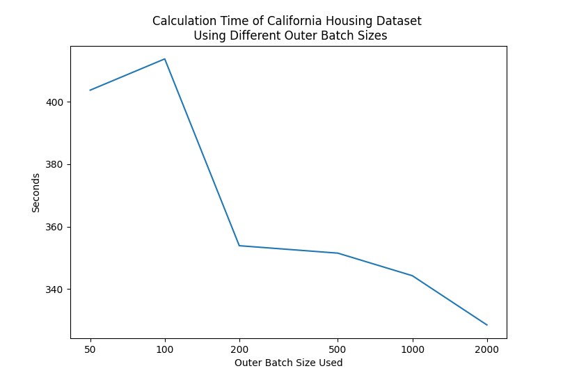
Increasing the outer batch size can have a significant effect on the run time of the process:

We will use the iris dataset for this example. Here, we load the data and train a simple lightgbm model on the dataset:

from sklearn.datasets import load_iris
import pandas as pd
import lightgbm as lgb
import numpy as np

# Define our dataset and target variable
data = pd.concat(load_iris(as_frame=True,return_X_y=True),axis=1)
data.rename({"target": "species"}, inplace=True, axis=1)
data["species"] = data["species"].astype("category")
target = data.pop("sepal length (cm)")

# Train our model
dtrain = lgb.Dataset(data=data, label=target)
lgbmodel = lgb.train(
    params={"seed": 1, "verbose": -1},
    train_set=dtrain,
    num_boost_round=10
)

# Define the function we wish to build shap values for.
model = lgbmodel.predict

preds = model(data)

We now have a model which takes a Pandas dataframe, and returns predictions. We can create an explainer that will use data as a background dataset to calculate the shap values of any dataset we wish:

from fastshap import KernelExplainer

ke = KernelExplainer(model, data)
sv = ke.calculate_shap_values(data, verbose=False)

print(all(preds == sv.sum(1)))

## True

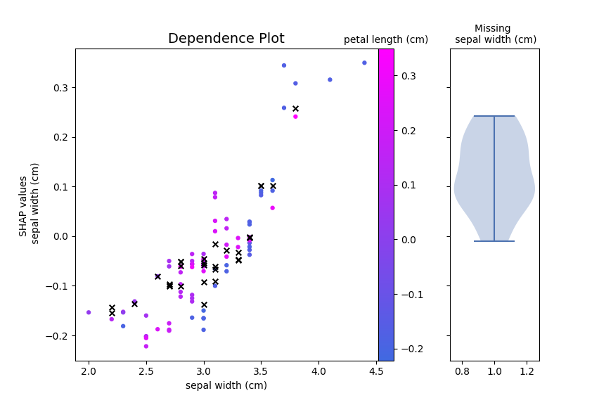
Dependence plots can be created by passing the shap values and variable / interaction information to plot_variable_effect_on_output:

from fastshap.plotting import plot_variable_effect_on_output
plot_variable_effect_on_output(
    sv, data,
    variable="sepal width (cm)",
    interaction_variable="auto"
)

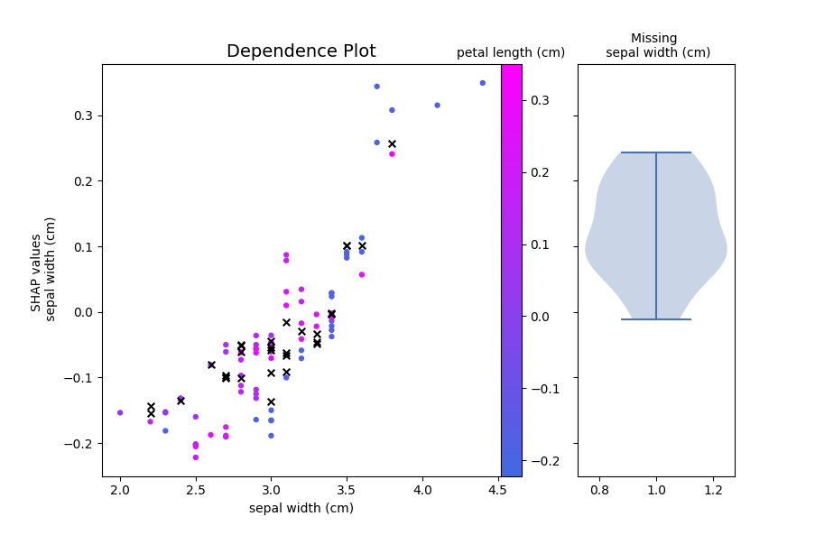
The type of plot that is generated depends on the model output, the variable type, and the interaction variable type. For example, plotting the effect of a categorical variable shows the following:

from fastshap.plotting import plot_variable_effect_on_output
plot_variable_effect_on_output(
    sv, data,
    variable="species",
    interaction_variable="auto"
)

We can select a subset of our data to act as a background set. By stratifying the background set on the results of the model output, we will usually get very similar results, while decreasing the caculation time drastically.

ke.stratify_background_set(5)
sv2 = ke.calculate_shap_values(
  data, 
  background_fold_to_use=0,
  verbose=False
)

print(np.abs(sv2 - sv).mean(0))

## [1.74764532e-03 1.61829094e-02 1.99534408e-03 4.02640884e-16
##  1.71084747e-02]

What we did is break up our background set into 10 different sets, stratified by the model output. We then used the first of these sets as our background set. We then compared the average difference between these shap values, and the shap values we obtained from using the entire dataset.

If the entire process was vectorized, it would require an array of size (# Samples * # Coalitions * # Background samples, # Columns). Where # Coalitions is the sum of the total number of coalitions that are going to be run. Even for small datasets, this becomes enormous. fastshap breaks this array up into chunks by splitting the process into a series of batches.

This is a list of the large arrays and their maximum size:

• Global
  • Mask Matrix (# Coalitions, # Columns)
• Outer Batch
  • Linear Targets (Total Coalition Combinations, Outer Batch Size, Output Dimension)`
• Inner Batch
  • Model Evaluation Features (Inner Batch Size, # Background Samples)`

The final, returned shap values will also be returned as the datatype returned by the model.

These theoretical sizes can be calculated directly so that the user can determine appropriate batch sizes for their machine:

# Combines our background data back into 1 DataFrame
ke.stratify_background_set(1)
(
    mask_matrix_size, 
    linear_target_size, 
    inner_model_eval_set_size
) = ke.get_theoretical_array_expansion_sizes(
    data=data,
    outer_batch_size=150,
    inner_batch_size=150,
    n_coalition_sizes=3,
    background_fold_to_use=None
)

print(
  np.product(linear_target_size) + np.product(inner_model_eval_set_size)
)

## 452100

For the iris dataset, even if we sent the entire set (150 rows) through as one batch, we only need 92100 elements stored in arrays. This is manageable on most machines. However, this number grows extremely quickly with the samples and number of columns. It is highly advised to determine a good batch scheme before running this process.

Another way to determine optimal batch sizes is to use the function .get_theoretical_minimum_memory_requirements(). This returns a list of Gigabytes needed to build the arrays above:

# Combines our background data back into 1 DataFrame
(
    mask_matrix_GB, 
    linear_target_GB, 
    inner_model_eval_set_GB
) = ke.get_theoretical_minimum_memory_requirements(
    data=data,
    outer_batch_size=150,
    inner_batch_size=150,
    n_coalition_sizes=3,
    background_fold_to_use=None
)

total_GB_needed = mask_matrix_GB + linear_target_GB + inner_model_eval_set_GB
print(f"We need {total_GB_needed} GB to calculate shap values with these batch sizes.")

## We need 0.003368459641933441 GB to calculate shap values with these batch sizes.

Any linear model available from sklearn.linear_model can be used to calculate the shap values. If you wish for some sparsity in the shap values, you can use Lasso regression:

from sklearn.linear_model import Lasso

# Use our entire background set
ke.stratify_background_set(1)
sv_lasso = ke.calculate_shap_values(
  data, 
  background_fold_to_use=0,
  linear_model=Lasso(alpha=0.1),
  verbose=False
)

print(sv_lasso[0,:])

## [-0.         -0.33797832 -0.         -0.14634971  5.84333333]

The default model used is sklearn.linear_model.LinearRegression.

If the model returns multiple outputs, the resulting shap values are returned as an array of size (rows, columns + 1, outputs). Therefore, to get the shap values for the effects on the second class, you need to slice the resulting shap values using shap_values[:,:,1]. Here is an example:

multi_features = pd.concat(load_iris(as_frame=True,return_X_y=True),axis=1)
multi_features.rename({"target": "species"}, inplace=True, axis=1)
target = multi_features.pop("species")

dtrain = lgb.Dataset(data=multi_features, label=target)
lgbmodel = lgb.train(
    params={"seed": 1, "objective": "multiclass", "num_class": 3, "verbose": -1},
    train_set=dtrain,
    num_boost_round=10
)
model = lgbmodel.predict

explainer_multi = KernelExplainer(model, multi_features)
shap_values_multi = explainer_multi.calculate_shap_values(multi_features, verbose=False)

# To get the shap values for the second class:
print(shap_values_multi.shape)

## (150, 5, 3)

Our shap values are a numpy array of shape (150, 5, 3) for each of our 150 rows, 4 columns (plus expected value), and our 3 output dimensions. When plotting multiclass outputs, the classes are essentially treated as a categorical variable. However, it is possible to plot variable interactions with one of the output classes, see below.
We can plot a variables shap values for each of the output classes:

plot_variable_effect_on_output(
    shap_values_multi,
    data,
    variable=2
)

We can also look at interactions if we are interested in a specific class. For instance, if we wanted to know the effect that sepal width (cm) had on our first class, we could do:

plot_variable_effect_on_output(sv, data, variable="sepal width (cm)", output_index=0)