Multiple Imputation with Random Forests in Python

Overview

Build Status Documentation Status MIT license CodeCov Code style: black
DEV_Version_Badge Pypi Conda Version PyVersions Downloads

miceforest: Fast, Memory Efficient Imputation with lightgbm

Fast, memory efficient Multiple Imputation by Chained Equations (MICE) with lightgbm. The R version of this package may be found here.

miceforest was designed to be:

  • Fast Uses lightgbm as a backend, and has efficient mean matching solutions.
  • Memory Efficient Capable of performing multiple imputation without copying the dataset. If the dataset can fit in memory, it can (probably) be imputed.
  • Flexible Can handle pandas DataFrames and numpy arrays. The imputation process can be completely customized. Can handle categorical data automatically.
  • Used In Production Kernels can be saved and impute new, unseen datasets. Imputing new data is often orders of magnitude faster than including the new data in a new mice procedure. Imputation models can be built off of a kernel dataset, even if there are no missing values. New data can also be imputed in place.

This document contains a thorough walkthrough of the package, benchmarks, and an introduction to multiple imputation. More information on MICE can be found in Stef van Buuren’s excellent online book, which you can find here.

Table of Contents:

Package Meta

News

New Major Update = 5.0.0

  • New main classes (ImputationKernel, ImputedData) replace (KernelDataSet, MultipleImputedKernel, ImputedDataSet, MultipleImputedDataSet).
  • Data can now be referenced and imputed in place. This saves a lot of memory allocation and is much faster.
  • Data can now be completed in place. This allows for only a single copy of the dataset to be in memory at any given time, even if performing multiple imputation.
  • mean_match_subset parameter has been replaced with data_subset. This subsets the data used to build the model as well as the candidates.
  • More performance improvements around when data is copied and where it is stored.
  • Raw data is now stored as the original. Can handle pandas DataFrame and numpy ndarray.

Installation

This package can be installed using either pip or conda, through conda-forge:

# Using pip
$ pip install miceforest --no-cache-dir

# Using conda
$ conda install -c conda-forge miceforest

You can also download the latest development version from this repository. If you want to install from github with conda, you must first run conda install pip git.

$ pip install git+https://github.com/AnotherSamWilson/miceforest.git

Classes

miceforest has 2 main classes which the user will interact with:

  • ImputationKernel - This class contains the raw data off of which the mice algorithm is performed. During this process, models will be trained, and the imputed (predicted) values will be stored. These values can be used to fill in the missing values of the raw data. The raw data can be copied, or referenced directly. Models can be saved, and used to impute new datasets.
  • ImputedData - The result of ImputationKernel.impute_new_data(new_data). This contains the raw data in new_data as well as the imputed values.

The Basics

We will be looking at a few simple examples of imputation. We need to load the packages, and define the data:

import miceforest as mf
from sklearn.datasets import load_iris
import pandas as pd
import numpy as np

# Load data and introduce missing values
iris = pd.concat(load_iris(as_frame=True,return_X_y=True),axis=1)
iris.rename({"target": "species"}, inplace=True, axis=1)
iris['species'] = iris['species'].astype('category')
iris_amp = mf.ampute_data(iris,perc=0.25,random_state=1991)

Basic Examples

If you only want to create a single imputed dataset, you can set the datasets parameter to 1:

# Create kernel. 
kds = mf.ImputationKernel(
  iris_amp,
  datasets=1,
  save_all_iterations=True,
  random_state=1991
)

# Run the MICE algorithm for 3 iterations
kds.mice(2)

There are also an array of plotting functions available, these are discussed below in the section Diagnostic Plotting.

We usually don’t want to impute just a single dataset. In statistics, multiple imputation is a process by which the uncertainty/other effects caused by missing values can be examined by creating multiple different imputed datasets. ImputationKernel can contain an arbitrary number of different datasets, all of which have gone through mutually exclusive imputation processes:

# Create kernel. 
kernel = mf.ImputationKernel(
  iris_amp,
  datasets=4,
  save_all_iterations=True,
  random_state=1
)

# Run the MICE algorithm for 2 iterations on each of the datasets
kernel.mice(2)

# Printing the kernel will show you some high level information.
print(kernel)
##               Class: ImputationKernel
##            Datasets: 4
##          Iterations: 2
##   Imputed Variables: 5
## save_all_iterations: True

After we have run mice, we can obtain our completed dataset directly from the kernel:

completed_dataset = kernel.complete_data(dataset=0, inplace=False)
print(completed_dataset.isnull().sum(0))
## sepal length (cm)    0
## sepal width (cm)     0
## petal length (cm)    0
## petal width (cm)     0
## species              0
## dtype: int64

Using inplace=False returns a copy of the completed data. Since the raw data is already stored in kernel.working_data, you can set inplace=True to complete the data without returning a copy:

kernel.complete_data(dataset=0, inplace=True)
print(kernel.working_data.isnull().sum(0))
## sepal length (cm)    0
## sepal width (cm)     0
## petal length (cm)    0
## petal width (cm)     0
## species              0
## dtype: int64

Controlling Tree Growth

Parameters can be passed directly to lightgbm in several different ways. Parameters you wish to apply globally to every model can simply be passed as kwargs to mice:

# Run the MICE algorithm for 1 more iteration on the kernel with new parameters
kernel.mice(iterations=1,n_estimators=50)

You can also pass pass variable-specific arguments to variable_parameters in mice. For instance, let’s say you noticed the imputation of the [species] column was taking a little longer, because it is multiclass. You could decrease the n_estimators specifically for that column with:

# Run the MICE algorithm for 2 more iterations on the kernel 
kernel.mice(iterations=1,variable_parameters={'species': {'n_estimators': 25}},n_estimators=50)

In this scenario, any parameters specified in variable_parameters takes presidence over the kwargs.

Preserving Data Assumptions

If your data contains count data, or any other data which can be parameterized by lightgbm, you can simply specify that variable to be modeled with the corresponding objective function. For example, let’s pretend sepal width (cm) is a count field which can be parameterized by a Poisson distribution:

# Create kernel. 
cust_kernel = mf.ImputationKernel(
  iris_amp,
  datasets=1,
  random_state=1
)

cust_kernel.mice(iterations=1, variable_parameters={'sepal width (cm)': {'objective': 'poisson'}})

Other nice parameters like monotone_constraints can also be passed.

Imputing with Gradient Boosted Trees

Since any arbitrary parameters can be passed to lightgbm.train(), it is possible to change the algrorithm entirely. This can be done simply like so:

# Create kernel. 
kds_gbdt = mf.ImputationKernel(
  iris_amp,
  datasets=1,
  save_all_iterations=True,
  random_state=1991
)

# We need to add a small minimum hessian, or lightgbm will complain:
kds_gbdt.mice(iterations=1, boosting='gbdt', min_sum_hessian_in_leaf=0.01)

# Return the completed kernel data
completed_data = kds_gbdt.complete_data(dataset=0)

Note: It is HIGHLY recommended to run parameter tuning if using gradient boosted trees. The parameter tuning process returns the optimal number of iterations, and usually results in much more useful parameter sets. See the section Tuning Parameters for more details.

Advanced Features

There are many ways to alter the imputation procedure to fit your specific dataset.

Customizing the Imputation Process

It is possible to heavily customize our imputation procedure by variable. By passing a named list to variable_schema, you can specify the predictors for each variable to impute. You can also specify mean_match_candidates and data_subset by variable by passing a dict of valid values, with variable names as keys. You can even replace the entire default mean matching function if you wish:

var_sch = {
    'sepal width (cm)': ['species','petal width (cm)'],
    'petal width (cm)': ['species','sepal length (cm)']
}
var_mmc = {
    'sepal width (cm)': 5,
    'petal width (cm)': 0
}
var_mms = {
  'sepal width (cm)': 50
}

# The mean matching function requires these parameters, even
# if it does not use them.
def mmf(
  mmc,
  model,
  candidate_features,
  bachelor_features,
  candidate_values,
  random_state
):

    bachelor_preds = model.predict(bachelor_features)
    imp_values = random_state.choice(candidate_values, size=bachelor_preds.shape[0])

    return imp_values

cust_kernel = mf.ImputationKernel(
    iris_amp,
    datasets=3,
    variable_schema=var_sch,
    mean_match_candidates=var_mmc,
    data_subset=var_mms,
    mean_match_function=mmf
)
cust_kernel.mice(1)

Imputing New Data with Existing Models

Multiple Imputation can take a long time. If you wish to impute a dataset using the MICE algorithm, but don’t have time to train new models, it is possible to impute new datasets using a ImputationKernel object. The impute_new_data() function uses the random forests collected by ImputationKernel to perform multiple imputation without updating the random forest at each iteration:

# Our 'new data' is just the first 15 rows of iris_amp
from datetime import datetime

# Define our new data as the first 15 rows
new_data = iris_amp.iloc[range(15)]

start_t = datetime.now()
new_data_imputed = kernel.impute_new_data(new_data=new_data)
print(f"New Data imputed in {(datetime.now() - start_t).total_seconds()} seconds")
## New Data imputed in 0.667865 seconds

All of the imputation parameters (variable_schema, mean_match_candidates, etc) will be carried over from the original ImputationKernel object. When mean matching, the candidate values are pulled from the original kernel dataset. To impute new data, the save_models parameter in ImputationKernel must be > 0. If save_models == 1, the model from the latest iteration is saved for each variable. If save_models > 1, the model from each iteration is saved. This allows for new data to be imputed in a more similar fashion to the original mice procedure.

Building Models on Nonmissing Data

The MICE process itself is used to impute missing data in a dataset. However, sometimes a variable can be fully recognized in the training data, but needs to be imputed later on in a different dataset. It is possible to train models to impute variables even if they have no missing values by setting train_nonmissing=True. In this case, variable_schema is treated as the list of variables to train models on. imputation_order only affects which variables actually have their values imputed, it does not affect which variables have models trained:

orig_missing_cols = ["sepal length (cm)", "sepal width (cm)"]
new_missing_cols = ["sepal length (cm)", "sepal width (cm)", "species"]

# Training data only contains 2 columns with missing data
iris_amp2 = iris.copy()
iris_amp2[orig_missing_cols] = mf.ampute_data(
  iris_amp2[orig_missing_cols],
  perc=0.25,
  random_state=1991
)

# Specify that models should also be trained for species column
var_sch = new_missing_cols

cust_kernel = mf.ImputationKernel(
    iris_amp2,
    datasets=1,
    variable_schema=var_sch,
    train_nonmissing=True
)
cust_kernel.mice(1)

# New data has missing values in species column
iris_amp2_new = iris.iloc[range(10),:].copy()
iris_amp2_new[new_missing_cols] = mf.ampute_data(
  iris_amp2_new[new_missing_cols],
  perc=0.25,
  random_state=1991
)

# Species column can still be imputed
iris_amp2_new_imp = cust_kernel.impute_new_data(iris_amp2_new)
iris_amp2_new_imp.complete_data(0).isnull().sum()
## sepal length (cm)    0
## sepal width (cm)     0
## petal length (cm)    0
## petal width (cm)     0
## species              0
## dtype: int64

Here, we knew that the species column in our new data would need to be imputed. Therefore, we specified that a model should be built for all 3 variables in the variable_schema (passing a dict of target - feature pairs would also have worked).

Tuning Parameters

miceforest allows you to tune the parameters on a kernel dataset. These parameters can then be used to build the models in future iterations of mice. In its most simple invocation, you can just call the function with the desired optimization steps:

# Using the first ImputationKernel in kernel to tune parameters
# with the default settings.
optimal_parameters, losses = kernel.tune_parameters(
  dataset=0,
  optimization_steps=5
)

# Run mice with our newly tuned parameters.
kernel.mice(1, variable_parameters=optimal_parameters)

# The optimal parameters are kept in ImputationKernel.optimal_parameters:
print(optimal_parameters)
## {0: {'boosting': 'gbdt', 'num_iterations': 65, 'max_depth': 8, 'num_leaves': 10, 'min_data_in_leaf': 1, 'min_sum_hessian_in_leaf': 0.1, 'min_gain_to_split': 0.0, 'bagging_fraction': 0.39791299065921537, 'feature_fraction': 1.0, 'feature_fraction_bynode': 0.6937388234549196, 'bagging_freq': 1, 'verbosity': -1, 'objective': 'regression', 'seed': 849382, 'learning_rate': 0.05, 'cat_smooth': 11.663587284343516}, 1: {'boosting': 'gbdt', 'num_iterations': 42, 'max_depth': 8, 'num_leaves': 13, 'min_data_in_leaf': 2, 'min_sum_hessian_in_leaf': 0.1, 'min_gain_to_split': 0.0, 'bagging_fraction': 0.35093507988596373, 'feature_fraction': 1.0, 'feature_fraction_bynode': 0.894341802252763, 'bagging_freq': 1, 'verbosity': -1, 'objective': 'regression', 'seed': 586321, 'learning_rate': 0.05, 'cat_smooth': 15.789844128272765}, 2: {'boosting': 'gbdt', 'num_iterations': 60, 'max_depth': 8, 'num_leaves': 7, 'min_data_in_leaf': 4, 'min_sum_hessian_in_leaf': 0.1, 'min_gain_to_split': 0.0, 'bagging_fraction': 0.9979861290119383, 'feature_fraction': 1.0, 'feature_fraction_bynode': 0.5730380093960374, 'bagging_freq': 1, 'verbosity': -1, 'objective': 'regression', 'seed': 961902, 'learning_rate': 0.05, 'cat_smooth': 20.39766682094556}, 3: {'boosting': 'gbdt', 'num_iterations': 61, 'max_depth': 8, 'num_leaves': 11, 'min_data_in_leaf': 6, 'min_sum_hessian_in_leaf': 0.1, 'min_gain_to_split': 0.0, 'bagging_fraction': 0.7560736024385001, 'feature_fraction': 1.0, 'feature_fraction_bynode': 0.8058628021146634, 'bagging_freq': 1, 'verbosity': -1, 'objective': 'regression', 'seed': 449169, 'learning_rate': 0.05, 'cat_smooth': 16.369979689010446}, 4: {'boosting': 'gbdt', 'num_iterations': 58, 'max_depth': 8, 'num_leaves': 18, 'min_data_in_leaf': 4, 'min_sum_hessian_in_leaf': 0.1, 'min_gain_to_split': 0.0, 'bagging_fraction': 0.5994031429682608, 'feature_fraction': 1.0, 'feature_fraction_bynode': 0.6270272146891186, 'bagging_freq': 1, 'verbosity': -1, 'objective': 'multiclass', 'num_class': 3, 'seed': 933848, 'learning_rate': 0.05, 'cat_smooth': 18.03460691618074}}

This will perform 10 fold cross validation on random samples of parameters. By default, all variables models are tuned. If you are curious about the default parameter space that is searched within, check out the miceforest.default_lightgbm_parameters module.

The parameter tuning is pretty flexible. If you wish to set some model parameters static, or to change the bounds that are searched in, you can simply pass this information to either the variable_parameters parameter, **kwbounds, or both:

# Using a complicated setup:
optimal_parameters, losses = kernel.tune_parameters(
  dataset=0,
  variables = ['sepal width (cm)','species','petal width (cm)'],
  variable_parameters = {
    'sepal width (cm)': {'bagging_fraction': 0.5},
    'species': {'bagging_freq': (5,10)}
  },
  optimization_steps=5,
  extra_trees = [True, False]
)

kernel.mice(1, variable_parameters=optimal_parameters)

In this example, we did a few things - we specified that only sepal width (cm), species, and petal width (cm) should be tuned. We also specified some specific parameters in variable_parameters. Notice that bagging_fraction was passed as a scalar, 0.5. This means that, for the variable sepal width (cm), the parameter bagging_fraction will be set as that number and not be tuned. We did the opposite for bagging_freq. We specified bounds that the process should search in. We also passed the argument extra_trees as a list. Since it was passed to **kwbounds, this parameter will apply to all variables that are being tuned. Passing values as a list tells the process that it should randomly sample values from the list, instead of treating them as set of counts to search within.

The tuning process follows these rules for different parameter values it finds:

  • Scalar: That value is used, and not tuned.
  • Tuple: Should be length 2. Treated as the lower and upper bound to search in.
  • List: Treated as a distinct list of values to try randomly.

How to Make the Process Faster

Multiple Imputation is one of the most robust ways to handle missing data - but it can take a long time. There are several strategies you can use to decrease the time a process takes to run:

  • Decrease data_subset. By default all non-missing datapoints for each variable are used to train the model and perform mean matching. This can cause the model training nearest-neighbors search to take a long time for large data. A subset of these points can be searched instead by using data_subset.
  • Convert your data to a numpy array. Numpy arrays are much faster to index. While indexing overhead is avoided as much as possible, there is no getting around it. Consider comverting to float32 datatype as well, as it will cause the resulting object to take up much less memory.
  • Decrease mean_match_candidates. The maximum number of neighbors that are considered with the default parameters is 10. However, for large datasets, this can still be an expensive operation. Consider explicitly setting mean_match_candidates lower.
  • Use different lightgbm parameters. lightgbm is usually not the problem, however if a certain variable has a large number of classes, then the max number of trees actually grown is (# classes) * (n_estimators). You can specifically decrease the bagging fraction or n_estimators for large multi-class variables, or grow less trees in general.
  • Use a faster mean matching function. The default mean matching function uses the scipy.Spatial.KDtree algorithm. There are faster alternatives out there, if you think mean matching is the holdup.

Imputing Data In Place

It is possible to run the entire process without copying the dataset. If copy_data=False, then the data is referenced directly:

kernel_inplace = mf.ImputationKernel(
  iris_amp,
  datasets=1,
  copy_data=False
)
kernel_inplace.mice(2)

Note, that this probably won’t (but could) change the original dataset in undesirable ways. Throughout the mice procedure, imputed values are stored directly in the original data. At the end, the missing values are put back as np.NaN.

We can also complete our original data in place:

kernel_inplace.complete_data(dataset=0, inplace=True)
print(iris_amp.isnull().sum(0))
## sepal length (cm)    0
## sepal width (cm)     0
## petal length (cm)    0
## petal width (cm)     0
## species              0
## dtype: int64

This is useful if the dataset is large, and copies can’t be made in memory.

Diagnostic Plotting

As of now, miceforest has four diagnostic plots available.

Distribution of Imputed-Values

We probably want to know how the imputed values are distributed. We can plot the original distribution beside the imputed distributions in each dataset by using the plot_imputed_distributions method of an ImputationKernel object:

kernel.plot_imputed_distributions(wspace=0.3,hspace=0.3)

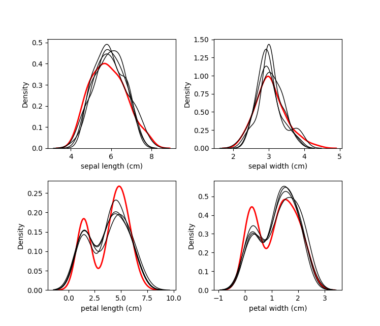
The red line is the original data, and each black line are the imputed values of each dataset.

Convergence of Correlation

We are probably interested in knowing how our values between datasets converged over the iterations. The plot_correlations method shows you a boxplot of the correlations between imputed values in every combination of datasets, at each iteration. This allows you to see how correlated the imputations are between datasets, as well as the convergence over iterations:

kernel.plot_correlations()

Variable Importance

We also may be interested in which variables were used to impute each variable. We can plot this information by using the plot_feature_importance method.

kernel.plot_feature_importance(dataset=0, annot=True,cmap="YlGnBu",vmin=0, vmax=1)

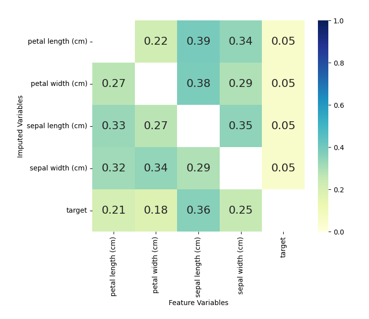
The numbers shown are returned from the lightgbm.Booster.feature_importance() function. Each square represents the importance of the column variable in imputing the row variable.

Mean Convergence

If our data is not missing completely at random, we may see that it takes a few iterations for our models to get the distribution of imputations right. We can plot the average value of our imputations to see if this is occurring:

kernel.plot_mean_convergence(wspace=0.3, hspace=0.4)

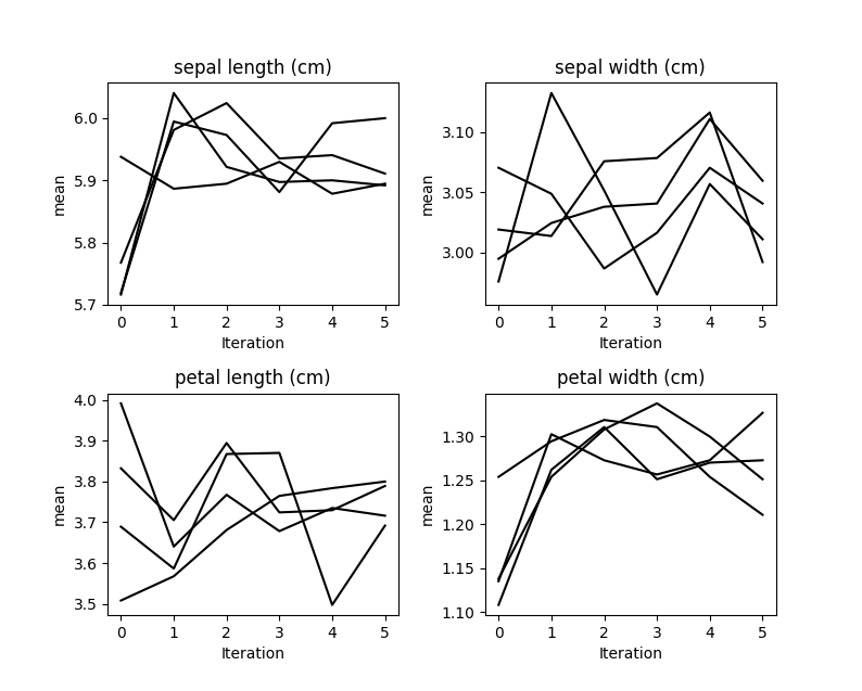
Our data was missing completely at random, so we don’t see any convergence occurring here.

Using the Imputed Data

To return the imputed data simply use the complete_data method:

dataset_1 = kernel.complete_data(0)

This will return a single specified dataset. Multiple datasets are typically created so that some measure of confidence around each prediction can be created.

Since we know what the original data looked like, we can cheat and see how well the imputations compare to the original data:

acclist = []
for iteration in range(kernel.iteration_count()+1):
    species_na_count = kernel.na_counts[4]
    compdat = kernel.complete_data(dataset=0,iteration=iteration)
    
    # Record the accuract of the imputations of species.
    acclist.append(
      round(1-sum(compdat['species'] != iris['species'])/species_na_count,2)
    )

# acclist shows the accuracy of the imputations
# over the iterations.
print(acclist)
## [0.35, 0.7, 0.78, 0.86, 0.84, 0.89, 0.84]

In this instance, we went from a ~32% accuracy (which is expected with random sampling) to an accuracy of ~65% after the first iteration. This isn’t the best example, since our kernel so far has been abused to show the flexability of the imputation procedure.

The MICE Algorithm

Multiple Imputation by Chained Equations ‘fills in’ (imputes) missing data in a dataset through an iterative series of predictive models. In each iteration, each specified variable in the dataset is imputed using the other variables in the dataset. These iterations should be run until it appears that convergence has been met.

This process is continued until all specified variables have been imputed. Additional iterations can be run if it appears that the average imputed values have not converged, although no more than 5 iterations are usually necessary.

Common Use Cases

Data Leakage:

MICE is particularly useful if missing values are associated with the target variable in a way that introduces leakage. For instance, let’s say you wanted to model customer retention at the time of sign up. A certain variable is collected at sign up or 1 month after sign up. The absence of that variable is a data leak, since it tells you that the customer did not retain for 1 month.

Funnel Analysis:

Information is often collected at different stages of a ‘funnel’. MICE can be used to make educated guesses about the characteristics of entities at different points in a funnel.

Confidence Intervals:

MICE can be used to impute missing values, however it is important to keep in mind that these imputed values are a prediction. Creating multiple datasets with different imputed values allows you to do two types of inference:

  • Imputed Value Distribution: A profile can be built for each imputed value, allowing you to make statements about the likely distribution of that value.
  • Model Prediction Distribution: With multiple datasets, you can build multiple models and create a distribution of predictions for each sample. Those samples with imputed values which were not able to be imputed with much confidence would have a larger variance in their predictions.

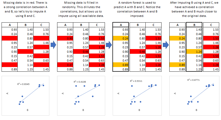
Predictive Mean Matching

miceforest can make use of a procedure called predictive mean matching (PMM) to select which values are imputed. PMM involves selecting a datapoint from the original, nonmissing data which has a predicted value close to the predicted value of the missing sample. The closest N (mean_match_candidates parameter) values are chosen as candidates, from which a value is chosen at random. This can be specified on a column-by-column basis. Going into more detail from our example above, we see how this works in practice:

This method is very useful if you have a variable which needs imputing which has any of the following characteristics:

  • Multimodal
  • Integer
  • Skewed

Effects of Mean Matching

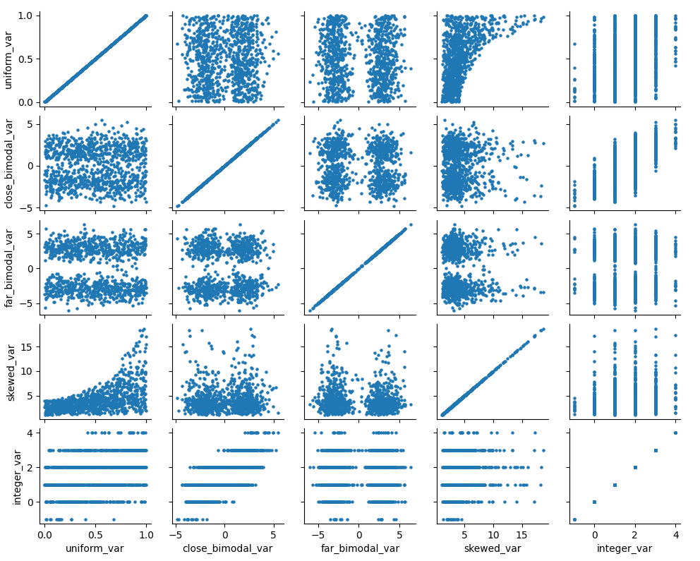
As an example, let’s construct a dataset with some of the above characteristics:

randst = np.random.RandomState(1991)
# random uniform variable
nrws = 1000
uniform_vec = randst.uniform(size=nrws)

def make_bimodal(mean1,mean2,size):
    bimodal_1 = randst.normal(size=nrws, loc=mean1)
    bimodal_2 = randst.normal(size=nrws, loc=mean2)
    bimdvec = []
    for i in range(size):
        bimdvec.append(randst.choice([bimodal_1[i], bimodal_2[i]]))
    return np.array(bimdvec)

# Make 2 Bimodal Variables
close_bimodal_vec = make_bimodal(2,-2,nrws)
far_bimodal_vec = make_bimodal(3,-3,nrws)


# Highly skewed variable correlated with Uniform_Variable
skewed_vec = np.exp(uniform_vec*randst.uniform(size=nrws)*3) + randst.uniform(size=nrws)*3

# Integer variable correlated with Close_Bimodal_Variable and Uniform_Variable
integer_vec = np.round(uniform_vec + close_bimodal_vec/3 + randst.uniform(size=nrws)*2)

# Make a DataFrame
dat = pd.DataFrame(
    {
    'uniform_var':uniform_vec,
    'close_bimodal_var':close_bimodal_vec,
    'far_bimodal_var':far_bimodal_vec,
    'skewed_var':skewed_vec,
    'integer_var':integer_vec
    }
)

# Ampute the data.
ampdat = mf.ampute_data(dat,perc=0.25,random_state=randst)

# Plot the original data
import seaborn as sns
import matplotlib.pyplot as plt
g = sns.PairGrid(dat)
g.map(plt.scatter,s=5)

We can see how our variables are distributed and correlated in the graph above. Now let’s run our imputation process twice, once using mean matching, and once using the model prediction.
kernelmeanmatch = mf.ImputationKernel(ampdat, datasets=1,mean_match_candidates=5)
kernelmodeloutput = mf.ImputationKernel(ampdat, datasets=1,mean_match_candidates=0)

kernelmeanmatch.mice(2)
kernelmodeloutput.mice(2)

Let’s look at the effect on the different variables.
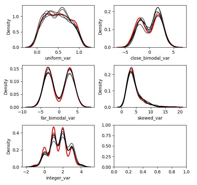
With Mean Matching
kernelmeanmatch.plot_imputed_distributions(wspace=0.2,hspace=0.4)

Without Mean Matching
kernelmodeloutput.plot_imputed_distributions(wspace=0.2,hspace=0.4)

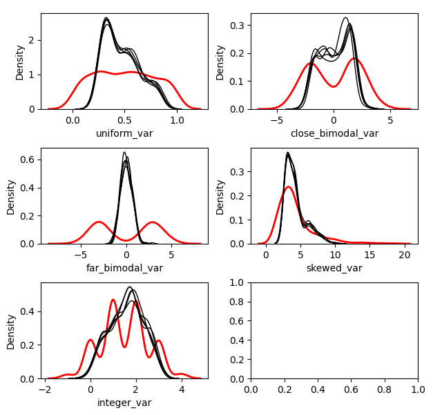
You can see the effects that mean matching has, depending on the distribution of the data. Simply returning the value from the model prediction, while it may provide a better ‘fit’, will not provide imputations with a similair distribution to the original. This may be beneficial, depending on your goal.

Comments
  • Using mean_match_candidates different from zero with categorical variables generates an error

    Using mean_match_candidates different from zero with categorical variables generates an error

    Hi,

    So other issue that I found using categorical variables imputation (category dtype) is that defining mean_match_candidates != 0 in Kernel definition generate an issue during .mice().

    Error message:

    /opt/conda/lib/python3.7/site-packages/miceforest/utils.py:377: RuntimeWarning: divide by zero encountered in true_divide
      odds_ratio = probability / (1 - probability)
    /opt/conda/lib/python3.7/site-packages/miceforest/utils.py:378: RuntimeWarning: divide by zero encountered in log
      log_odds = np.log(odds_ratio)
    ---------------------------------------------------------------------------
    KeyError                                  Traceback (most recent call last)
    <ipython-input-106-6f8a47b02d4b> in <module>
          9                                    mean_match_candidates=2)
         10 # Run the MICE algorithm for X iterations - 12:09 - 13:22
    ---> 11 a.mice(iterations=2, verbose=True, n_jobs=-1)
    
    /opt/conda/lib/python3.7/site-packages/miceforest/ImputationKernel.py in mice(self, iterations, verbose, variable_parameters, compile_candidates, **kwlgb)
       1193                                 random_state=self._random_state,
       1194                                 hashed_seeds=None,
    -> 1195                                 candidate_preds=candidate_preds,
       1196                             )
       1197                         )
    
    /opt/conda/lib/python3.7/site-packages/miceforest/mean_match_schemes.py in mean_match_function_kdtree_cat(mmc, model, bachelor_features, candidate_values, random_state, hashed_seeds, candidate_preds)
        361                 candidate_values,
        362                 random_state,
    --> 363                 hashed_seeds,
        364             )
        365 
    
    /opt/conda/lib/python3.7/site-packages/miceforest/mean_match_schemes.py in _mean_match_multiclass_accurate(mmc, bachelor_preds, candidate_preds, candidate_values, random_state, hashed_seeds)
        119 
        120     index_choice = knn_indices[np.arange(knn_indices.shape[0]), ind]
    --> 121     imp_values = candidate_values[index_choice]
        122 
        123     return imp_values
    
    /opt/conda/lib/python3.7/site-packages/pandas/core/series.py in __getitem__(self, key)
        964             return self._get_values(key)
        965 
    --> 966         return self._get_with(key)
        967 
        968     def _get_with(self, key):
    
    /opt/conda/lib/python3.7/site-packages/pandas/core/series.py in _get_with(self, key)
        999             #  (i.e. self.iloc) or label-based (i.e. self.loc)
       1000             if not self.index._should_fallback_to_positional():
    -> 1001                 return self.loc[key]
       1002             else:
       1003                 return self.iloc[key]
    
    /opt/conda/lib/python3.7/site-packages/pandas/core/indexing.py in __getitem__(self, key)
        929 
        930             maybe_callable = com.apply_if_callable(key, self.obj)
    --> 931             return self._getitem_axis(maybe_callable, axis=axis)
        932 
        933     def _is_scalar_access(self, key: tuple):
    
    /opt/conda/lib/python3.7/site-packages/pandas/core/indexing.py in _getitem_axis(self, key, axis)
       1151                     raise ValueError("Cannot index with multidimensional key")
       1152 
    -> 1153                 return self._getitem_iterable(key, axis=axis)
       1154 
       1155             # nested tuple slicing
    
    /opt/conda/lib/python3.7/site-packages/pandas/core/indexing.py in _getitem_iterable(self, key, axis)
       1091 
       1092         # A collection of keys
    -> 1093         keyarr, indexer = self._get_listlike_indexer(key, axis)
       1094         return self.obj._reindex_with_indexers(
       1095             {axis: [keyarr, indexer]}, copy=True, allow_dups=True
    
    /opt/conda/lib/python3.7/site-packages/pandas/core/indexing.py in _get_listlike_indexer(self, key, axis)
       1312             keyarr, indexer, new_indexer = ax._reindex_non_unique(keyarr)
       1313 
    -> 1314         self._validate_read_indexer(keyarr, indexer, axis)
       1315 
       1316         if needs_i8_conversion(ax.dtype) or isinstance(
    
    /opt/conda/lib/python3.7/site-packages/pandas/core/indexing.py in _validate_read_indexer(self, key, indexer, axis)
       1375 
       1376             not_found = list(ensure_index(key)[missing_mask.nonzero()[0]].unique())
    -> 1377             raise KeyError(f"{not_found} not in index")
       1378 
       1379 
    
    KeyError: '[129846] not in index'
    

    What I found is that using the default of mean_matching_scheme parameter was causing the issue (because will evaluate for categorical features the Mean Matching) and that using miceforest.mean_match_schemes.mean_match_scheme_fast_cat was turning around for that.

    opened by KaikeWesleyReis 26
  • Column types are not the same as the original data. Check categorical columns.

    Column types are not the same as the original data. Check categorical columns.

    Hey, I tried to implement a missing imputation process splitting the data into x_train, x_test and x_val. This error came up and I don't know exactly what it means. I checked the data types of the columns of the three datasets( x_train, x_test and x_val), and they are the same.

    AssertionError: Column types are not the same as the original data. Check categorical columns.

    opened by Ededu1984 10
  • Workaround to

    Workaround to " __init__() got an unexpected keyword argument 'balanced_tree' "

    Awesome library! From prior posts it seems like the error "init() got an unexpected keyword argument 'balanced_tree' " is related to scipy. In the meantime before scipy is updated, is there any workaround/hack?

    opened by agt64 10
  • IndexError using impute_new_data

    IndexError using impute_new_data

    I am trying to impute new data using the kernel.

    from datetime import datetime
    
    start_t = datetime.now()
    new_data_imputed = kernel.impute_new_data(new_data=new_sub)
    print(f"New Data imputed in {(datetime.now() - start_t).total_seconds()} seconds")


    But, I keep getting an IndexError:

    ---------------------------------------------------------------------------
    IndexError                                Traceback (most recent call last)
    /var/folders/36/j_203fcj42q9bvnlt1sl3j640000gp/T/ipykernel_54504/3730750411.py in <module>
          2 
          3 start_t = datetime.now()
    ----> 4 new_data_imputed = kernel.impute_new_data(new_data=new_sub)
          5 print(f"New Data imputed in {(datetime.now() - start_t).total_seconds()} seconds")
    
    ~/.pyenv/versions/3.8.3/lib/python3.8/site-packages/miceforest/ImputationKernel.py in impute_new_data(self, new_data, datasets, iterations, save_all_iterations, copy_data, random_state, verbose)
       1233                         )
       1234                     )
    -> 1235                     imputed_data._insert_new_data(
       1236                         dataset=ds, variable_index=var, new_data=imp_values
       1237                     )
    
    ~/.pyenv/versions/3.8.3/lib/python3.8/site-packages/miceforest/ImputedData.py in _insert_new_data(self, dataset, variable_index, new_data)
        387         view = _slice(self.working_data, col_slice=variable_index)
        388         if view.dtype.name == "category":
    --> 389             new_data = np.array(view.cat.categories)[new_data]
        390 
        391         _assign_col_values_without_copy(
    
    IndexError: index 1 is out of bounds for axis 0 with size 1
    

    Shape of original data: (33008, 71) Shape of new_sub: (15, 71) Both datasets have columns that are all of the same data type. What could be causing this issue?

    opened by mjoy296 7
  • Potentially incorrect imputations depending on feature order in variable schema

    Potentially incorrect imputations depending on feature order in variable schema

    Hi,

    I noticed an unexpected imputation behaviour that can be illustrated with the following example:

    • I create three independent (uncorrelated) features f0, f1 and f2. Features f0 and f2 are Gaussian, f1 is Exponential. Furthermore, f1 and f2 have clearly different means.
    • I induce missingness completely at random in feature f0, and then use f1 and f2 to impute it.
    • If I specify a variable schema {'f0':['f2, 'f1']}, then imputed values are too low.
    • If I specify a schema {'f0':['f1, 'f2']}, then imputed values are as expected.
    • This behaviour happens when f2 and f1 have different means. It also occurs when features f1 and f2 are Gaussian, but is more clear when one is exponential.

    The order of f1 and f2 should not matter, because there are no missing values in these features. It should also not matter because f1 and f2 carry no information about f0. I wonder if this could be a bug? I hope I have not overlooked anything obvious!

    Thanks, Andres

    Code to illustrate this:

    # Get data with three independent features - f0,f1,f2
    # f0 and f2 are Gaussian, f1 is Exponential
    n = 1000
    rng0 = np.random.default_rng(seed=42)
    rng1 = np.random.default_rng(seed=52)
    rng2 = np.random.default_rng(seed=62)
    f0 = rng0.normal(loc=0, scale=1, size=n)
    f1 = rng1.exponential(scale=1, size=n)
    f2 = rng2.normal(loc=10, scale=1, size=n)
    plt.hist(f0, alpha=0.5, label='Feature 0')
    plt.hist(f1, alpha=0.5, label='Feature 1')
    plt.hist(f2, alpha=0.5, label='Feature 2')
    plt.legend()
    plt.show()
    d = np.vstack([f0,f1,f2]).transpose()
    d = pd.DataFrame(d, columns=['f0', 'f1', 'f2'])
    print('\nDataset:\n{}'.format(d.describe()))
    
    # Induce missingness completely at random in feature 0
    idx_mis = rng.choice(np.arange(n), int(np.floor(n/2)))
    d.iloc[idx_mis,0] = np.nan
    
    # Impute: f2 before f1 in schema - not good result
    # Imputed values are lower than the mean
    var_sch = {'f0':['f2', 'f1']}
    print('\nVariable schema: {}'.format(var_sch))
    kernel = mf.ImputationKernel(d, datasets=1, random_state=42, 
                                 mean_match_scheme=mean_match_default,
                                 variable_schema=var_sch)
    kernel.mice(5)
    d_imp = kernel.complete_data(0)
    d_imp = pd.concat(objs=[d_imp.f0, d.f0], axis=1)
    d_imp.columns = ['f0 (imputed)', 'f0']
    print('Distribution of imputed feature vs unimputed feature:\n\n{}'.format(d_imp.describe()))
    kernel.plot_imputed_distributions(wspace=1,hspace=0.5)
    
    # Impute: f1 before f2 in schema - good result
    var_sch = {'f0':['f1', 'f2']}
    print('\nVariable schema: {}'.format(var_sch))
    kernel = mf.ImputationKernel(d, datasets=1, random_state=42, 
                                 mean_match_scheme=mean_match_default,
                                 variable_schema=var_sch)
    kernel.mice(5)
    d_imp = kernel.complete_data(0)
    d_imp = pd.concat(objs=[d_imp.f0, d.f0], axis=1)
    d_imp.columns = ['f0 (imputed)', 'f0']
    print('Distribution of imputed feature vs unimputed feature:\n\n{}'.format(d_imp.describe()))
    kernel.plot_imputed_distributions(wspace=1,hspace=0.5)
    

    Output I get on my computer (without plots):

    Dataset:
                    f0           f1           f2
    count  1000.000000  1000.000000  1000.000000
    mean     -0.028892     0.933777     9.987793
    std       0.989217     0.951335     0.968862
    min      -3.648413     0.000646     7.231604
    25%      -0.696313     0.285916     9.253244
    50%       0.006178     0.648893    10.026187
    75%       0.589887     1.216675    10.637074
    max       3.178854     7.129019    13.086357
    
    Variable schema: {'f0': ['f2', 'f1']}
    Distribution of imputed feature vs unimputed feature:
    
           f0 (imputed)          f0
    count   1000.000000  599.000000
    mean      -0.883467   -0.011545
    std        1.337261    1.007416
    min       -2.964529   -2.964529
    25%       -1.861845   -0.690939
    50%       -1.033285   -0.005122
    75%        0.221387    0.638580
    max        2.905067    2.905067
    
    Variable schema: {'f0': ['f1', 'f2']}
    Distribution of imputed feature vs unimputed feature:
    
           f0 (imputed)          f0
    count   1000.000000  599.000000
    mean       0.006233   -0.011545
    std        0.977652    1.007416
    min       -2.964529   -2.964529
    25%       -0.654283   -0.690939
    50%        0.011445   -0.005122
    75%        0.637487    0.638580
    max        2.905067    2.905067
    
    opened by tammandres 5
  • On the use of categorical variables

    On the use of categorical variables

    First of all, really good library, I find it quite useful and easy to implement.The problem is I am not able to use it on categorical variables as you claim it can be done. I can only encode them in such a way that I can use the imputation as if they were numerical variables (using OHE or similar techniques).

    Could you add a section on the read.me as to how to use MICE Forest with categorical variables?

    opened by CarlosHernandezP 5
  • How to customize initial imputations

    How to customize initial imputations

    Hello! Very useful project! I think proper initial imputation will improve the final imputation accuracy of the model, so I want to customize the initial imputation method. Now, I want to customize an initial imputation method, but I don't know how to modify the code. I hope to get some help and look forward to your reply.

    opened by MrWeijing 3
  • AssertionError mean_match_candidate > data_subset

    AssertionError mean_match_candidate > data_subset

    The data look very normal so not sure what is happening image

    import miceforest as mf
    
    scheme_mms_5 =mf.mean_match_shap.copy()
    scheme_mms_5.set_mean_match_candidates(1)
    
    kds = mf.ImputationKernel(
    X_train,
    mean_match_scheme=scheme_mms_5,
    datasets=1,
    save_all_iterations=True,
    # train_nonmissing=True, #even if not missing now, maybe future
    save_models=1,
    # data_subset=1000,
    random_state=1991)
    
    # kds = mf.ImputationKernel(X_train)
    
    # Run the MICE algorithm for 1 iterations
    kds.mice(2, verbose=True)
    
    completed_dataset = kds.complete_data(dataset=0, inplace=False)
    completed_dataset  = pd.DataFrame(completed_dataset, index=X_train.index, columns=X_train.columns)
    
    ---------------------------------------------------------------------------
    
    AssertionError                            Traceback (most recent call last)
    
    [<ipython-input-72-038010c0385d>](https://localhost:8080/#) in <module>
         12 save_models=1,
         13 # data_subset=1000,
    ---> 14 random_state=1991)
         15 
         16 # kds = mf.ImputationKernel(X_train)
    
    [/usr/local/lib/python3.7/dist-packages/miceforest/ImputationKernel.py](https://localhost:8080/#) in __init__(self, data, datasets, variable_schema, imputation_order, train_nonmissing, mean_match_scheme, data_subset, categorical_feature, initialization, save_all_iterations, save_models, copy_data, save_loggers, random_state)
        343         for v in self.imputation_order:
        344             mmc = self.mean_match_scheme.mean_match_candidates[v]
    --> 345             assert mmc <= data_subset[v], f"{v} mean_match_candidates > data_subset"
        346             assert (
        347                 data_subset[v] <= available_candidates[v]
    
    AssertionError: 142 mean_match_candidates > data_subset
    
    opened by firmai 3
  • Could you add skip columns?

    Could you add skip columns?

    Hi :) I'm big fan of this library!

    I'm trying to change source code to make it run in the way I want, but it is not that easy :(

    I'm currently working on Kaggle competition with huge size of dataset including missing values.

    Although this nice library and LGBM is pretty fast, but I want to fill columns which only have missing values, not for all columns.

    my suggestion is adding list to specify columns in mice method.

    instead of

    for variable in self.variable_training_order:
    

    put new variable

    for var in self.variable_people_select
    

    Also I'm wondering just adding one parameter to mice method, like,

        def mice(
            self,
            iterations=2,
            verbose=False,
            variable_parameters=None,
            compile_candidates=False,
            user_specified_columns=None, <- 
            **kwlgb,
        ):
    

    Thank you for your awesome library ;)

    opened by keonho-kim 3
  • New Data Imputation issue arise when using train_nonmissing as True

    New Data Imputation issue arise when using train_nonmissing as True

    Hi, First, congratulations for your package @AnotherSamWilson !

    I'm facing an issue related to the ImputedData object: When I use train_nonmissing=True in Kernel definition, I have an error with the returned object from impute_new_data, but I'm still able to do the imputation by calling the complete_data function.

    I prepared an example using the same dataset from your README.md. When I use the Kernel definition as you presented, i.e. train_nonmissing=False:

    import miceforest as mf
    from sklearn.datasets import load_iris
    # Load data and introduce missing values
    iris = pd.concat(load_iris(as_frame=True,return_X_y=True),axis=1)
    iris.rename({"target": "species"}, inplace=True, axis=1)
    iris['species'] = iris['species'].astype('category')
    iris_amp = mf.ampute_data(iris,perc=0.25,random_state=1991)
    # Create kernel. 
    kds = mf.ImputationKernel(iris_amp, datasets=1, save_all_iterations=True, train_nonmissing=False, random_state=1991)
    # Run the MICE algorithm for 2 iterations
    kds.mice(2)
    
    # Return the completed dataset -> Just works normally
    iris_complete = kds.complete_data(0)
    #print(iris_complete.isnull().sum())
    # New data has missing values in species column
    new_missing_cols = ["sepal length (cm)", "sepal width (cm)", "species"]
    iris_amp2_new = iris.iloc[range(10),:].copy()
    iris_amp2_new[new_missing_cols] = mf.ampute_data(iris_amp2_new[new_missing_cols], perc=0.25,random_state=1991)
    
    # Species column can still be imputed
    iris_amp2_new_imp = kds.impute_new_data(iris_amp2_new)
    iris_amp2_new_imp.complete_data(0).isnull().sum()
    

    I have the following result: good-result

    But, this exactly same code with train_nonmissing=True generates this: bad-result

    For the complete log error:

    ---------------------------------------------------------------------------
    ValueError                                Traceback (most recent call last)
    /opt/conda/lib/python3.7/site-packages/IPython/core/formatters.py in __call__(self, obj)
        700                 type_pprinters=self.type_printers,
        701                 deferred_pprinters=self.deferred_printers)
    --> 702             printer.pretty(obj)
        703             printer.flush()
        704             return stream.getvalue()
    
    /opt/conda/lib/python3.7/site-packages/IPython/lib/pretty.py in pretty(self, obj)
        392                         if cls is not object \
        393                                 and callable(cls.__dict__.get('__repr__')):
    --> 394                             return _repr_pprint(obj, self, cycle)
        395 
        396             return _default_pprint(obj, self, cycle)
    
    /opt/conda/lib/python3.7/site-packages/IPython/lib/pretty.py in _repr_pprint(obj, p, cycle)
        698     """A pprint that just redirects to the normal repr function."""
        699     # Find newlines and replace them with p.break_()
    --> 700     output = repr(obj)
        701     lines = output.splitlines()
        702     with p.group():
    
    /opt/conda/lib/python3.7/site-packages/miceforest/ImputedData.py in __repr__(self)
        339 
        340     def __repr__(self):
    --> 341         summary_string = " " * 14 + "Class: ImputedData\n" + self._ids_info()
        342         return summary_string
        343 
    
    /opt/conda/lib/python3.7/site-packages/miceforest/ImputedData.py in _ids_info(self)
        347          Iterations: {self.iteration_count()}
        348   Imputed Variables: {len(self.imputation_order)}
    --> 349 save_all_iterations: {self.save_all_iterations}"""
        350         return summary_string
        351 
    
    /opt/conda/lib/python3.7/site-packages/miceforest/ImputedData.py in iteration_count(self, datasets, variables)
        498         if len(ds_uniq) > 1:
        499             raise ValueError(
    --> 500                 "iterations were not consistent across provided datasets, variables."
        501             )
        502 
    
    ValueError: iterations were not consistent across provided datasets, variables.
    

    From my research around your code, my suspicion is if I don't have to impute a nonmissing column, this error would happen, but my tests shows that this wasn't the issue. The object fails given a check from the model.

    How could I fix this?

    opened by KaikeWesleyReis 3
  • i cannot run    kds.mice(2)

    i cannot run kds.mice(2)

    D:\anaconda\lib\site-packages\lightgbm\engine.py:239: UserWarning: 'verbose_eval' argument is deprecated and will be removed in a future release of LightGBM. Pass 'log_evaluation()' callback via 'callbacks' argument instead. _log_warning("'verbose_eval' argument is deprecated and will be removed in a future release of LightGBM. " D:\anaconda\lib\site-packages\lightgbm\basic.py:1491: UserWarning: 'silent' argument is deprecated and will be removed in a future release of LightGBM. Pass 'verbose' parameter via 'params' instead. _log_warning("'silent' argument is deprecated and will be removed in a future release of LightGBM. "

    TypeError Traceback (most recent call last) in ----> 1 kds.mice(2)

    D:\anaconda\lib\site-packages\miceforest\ImputationKernel.py in mice(self, iterations, verbose, variable_parameters, **kwlgb) 844 ) 845 imp_values = np.array( --> 846 self.mean_match_function( 847 mmc=self.mean_match_candidates[var], 848 model=current_model,

    D:\anaconda\lib\site-packages\miceforest\mean_matching_functions.py in default_mean_match(mmc, model, candidate_features, bachelor_features, candidate_values, random_state) 108 # balanced_tree = False fixes a recursion issue for some reason. 109 # https://github.com/scipy/scipy/issues/14799 --> 110 kd_tree = KDTree(candidate_preds, leafsize=16, balanced_tree=False) 111 _, knn_indices = kd_tree.query(bachelor_preds, k=mmc, workers=-1) 112

    TypeError: init() got an unexpected keyword argument 'balanced_tree'

    opened by ccd545235100 3
  • Pandas dtypes modified when predicting on single records

    Pandas dtypes modified when predicting on single records

    Hi,

    We encountered several issues when we tried to impute new dataset with one or few records. We ensured to convert the input dataset to the same types as we had during training, but we still get:

    ValueError: train and valid dataset categorical_feature do not match.

    After some investigations, we found out that dtypes of input data can change in the function _assign_col_values_without_copy from utils. We applied a quick and dirty fix on our side:

    def _assign_col_values_without_copy(dat, row_ind, col_ind, val):
        """
        Insert values into different data frame objects.
        """
        row_ind = _ensure_iterable(row_ind)
        dtype_bef = dat.iloc[:, col_ind].dtype
        if isinstance(dat, pd_DataFrame):
            dat.iloc[row_ind, col_ind] = val
            dtype_aft = dat.iloc[:, col_ind].dtype
            # Keep same dtype after values assignment
            if dtype_bef != dtype_aft:
                dat.iloc[:, col_ind] = dat.iloc[:, col_ind].astype(dtype_bef)
        elif isinstance(dat, np.ndarray):
            dat[row_ind, col_ind] = val
        else:
            raise ValueError("Unknown data class passed.")
    

    It works now on individual predictions but we wanted to get your thoughts about that potential fix.

    Thanks for your help!

    opened by getchepare2 11
  • Compile predictions optimaly before impute_new_data is called

    Compile predictions optimaly before impute_new_data is called

    If save_models == 1, procedure will be fastest and use least memory when predictions are compiled and deleted at the start/end of imputations for each dataset.

    enhancement 
    opened by AnotherSamWilson 0
  • Imputed values differ after a kernel is loaded

    Imputed values differ after a kernel is loaded

    Hi @AnotherSamWilson,

    The related issue is the fact that for large dataset (my case at least) the imputed values for the same dataset differ before (trained kernel) and after (that same kernel saved and loaded) the imputation. The example bellow show what I'm talking:

    image

    Here 2% was different from one set to another.

    I'll reproduce this same idea with Iris dataset to verify.

    opened by KaikeWesleyReis 7
Releases(DOI)
  • DOI(Dec 12, 2022)

  • v5.6.0(Jul 29, 2022)

    This release implemented some major changes:

    • Implemented MeanMatchScheme
    • Implemented mean matching on shap values
    • Tighter controls and warnings around categorical levels
    • Included type hints for major functions.

    This release is marked as stable because the API will not see significant changes in the future.

    Source code(tar.gz)
    Source code(zip)
  • v5.0.0(Oct 15, 2021)

    • New main classes (ImputationKernel, ImputedData) replace (ImputationKernel, ImputationKernel, ImputedDataSet, MultipleImputedDataSet).
    • Data can now be referenced and imputed in place. This saves a lot of memory allocation and is much faster.
    • Data can now be completed in place. This allows for only a single copy of the dataset to be in memory at any given time, even if performing multiple imputation.
    • mean_match_subset parameter has been replaced with data_subset. This subsets the data used to build the model as well as the candidates.
    • More performance improvements around when data is copied and where it is stored.
    • Raw data is now stored as the original. Can handle pandas DataFrame and numpy ndarray.
    Source code(tar.gz)
    Source code(zip)
  • V4.0.0(Sep 28, 2021)

    This release improved a number of areas:

    • Huge performance improvements, especially if categorical variables were being imputed. These come from not predicting candidate data if we don't need to, using a much faster neighbors search, using numpy internally for indexing instead of pandas, and others.
    • Ability to tune parameters of models, and use best parameters for mice.
    • Improvements to code layout - got rid of ImputationSchema.
    • Raw data is now stored as a numpy array to save space and improve indexing.
    • Numpy arrays can be imputed, if you want to avoid pandas.
    • Options of multiple build-in mean matching functions.
    • Mean matching functions can handle most lightgbm objectives.
    Source code(tar.gz)
    Source code(zip)
  • v3.0.0(Sep 3, 2021)

    This is a major release, with breaking API changes:

    • The random forest package is now lightgbm
      • Much more lightweight (serialized kernels tend to be 5x smaller or more)
      • Much faster on big datasets (for comparable parameters)
      • More flexible... We can now use gbdt if we wish. lightgbm is more flexible in general.
    • Added a mean_match_subset parameter. This will help greatly speed up many processes.
    • mean_match_candidates now lazily accepts dicts as long as the keys are a subset of parameters in variable_schema.
    • Model parameters can be specified by variable, or globally.
    • Mean matching function can be overwritten if the user wishes.
    Source code(tar.gz)
    Source code(zip)
  • v2.0.1(Sep 8, 2020)

    • Models from all iterations can be saved with save_models == 2.
    • Kernel classes inherit from base imputed classes - allows for methods to be called on imputed datasets obtained form impute_new_data().
    • Time log was added
    • MultipleImputedDataset is now a collection of ImputedDataSets with methods for comparing them. Subscripting gives the desired dataset.
    • Tests updated to be much more comprehensive
    • Datasets can now be added and removed from a MultipleImputedDataSet/MultipleImputedKernel.
    Source code(tar.gz)
    Source code(zip)
  • v1.0.8(Aug 31, 2020)

Owner
Samuel Wilson
Samuel Wilson
Search algorithm implementations meant for teaching

Search-py A collection of search algorithms for teaching and experimenting. Non-adversarial Search There’s a heavy separation of concerns which leads

Dietrich Daroch 5 Mar 07, 2022
A simple python implementation of A* and bfs algorithm solving Eight-Puzzle

A simple python implementation of A* and bfs algorithm solving Eight-Puzzle

2 May 22, 2022
Python sample codes for robotics algorithms.

PythonRobotics Python codes for robotics algorithm. Table of Contents What is this? Requirements Documentation How to use Localization Extended Kalman

Atsushi Sakai 17.2k Jan 01, 2023
A python implementation of the Basic Photometric Stereo Algorithm

Photometric-Stereo A python implementation of the Basic Photometric Stereo Algorithm Result Usage run Photometric_Stereo.py Code Tree |data #原始数据,tga格

20 Dec 19, 2022
Leveraging Unique CPS Properties to Design Better Privacy-Enhancing Algorithms

Differential_Privacy_CPS Python implementation of the research paper Leveraging Unique CPS Properties to Design Better Privacy-Enhancing Algorithms Re

Shubhesh Anand 2 Dec 14, 2022
Machine Learning algorithms implementation.

Machine Learning Algorithms Machine Learning algorithms implementation. What can I find here? ML Algorithms KNN K-Means-Clustering SVM (MultiClass) Pe

David Levin 1 Dec 10, 2021
My own Unicode compression algorithm

Zee Code ZCode is a custom compression algorithm I originally developed for a competition held for the Spring 2019 Datastructures and Algorithms cours

Vahid Zehtab 2 Oct 20, 2021
This project is an implementation of a simple K-means algorithm

Simple-Kmeans-Clustering-Algorithm Abstract K-means is a centroid-based algorithm, or a distance-based algorithm, where we calculate the distances to

Saman Khamesian 7 Aug 09, 2022
Infomap is a network clustering algorithm based on the Map equation.

Infomap Infomap is a network clustering algorithm based on the Map equation. For detailed documentation, see mapequation.org/infomap. For a list of re

347 Dec 23, 2022
Algorithms and utilities for SAR sensors

WARNING: THIS CODE IS NOT READY FOR USE Sarsen Algorithms and utilities for SAR sensors Objectives Be faster and simpler than ESA SNAP and cloud nativ

B-Open 201 Dec 27, 2022
A tictactoe where you never win, implemented using minimax algorithm

Unbeatable_TicTacToe A tictactoe where you never win, implemented using minimax algorithm Requirements Make sure you have the pygame module along with

Jessica Jolly 3 Jul 28, 2022
GoldenSAML Attack Libraries and Framework

WhiskeySAML and Friends TicketsPlease TicketsPlease: Python library to assist with the generation of Kerberos tickets, remote retrieval of ADFS config

Secureworks 43 Jan 03, 2023
A lightweight, object-oriented finite state machine implementation in Python with many extensions

transitions A lightweight, object-oriented state machine implementation in Python with many extensions. Compatible with Python 2.7+ and 3.0+. Installa

4.7k Jan 01, 2023
zoofs is a Python library for performing feature selection using an variety of nature inspired wrapper algorithms. The algorithms range from swarm-intelligence to physics based to Evolutionary. It's easy to use ,flexible and powerful tool to reduce your feature size.

zoofs is a Python library for performing feature selection using a variety of nature-inspired wrapper algorithms. The algorithms range from swarm-intelligence to physics-based to Evolutionary. It's e

Jaswinder Singh 168 Dec 30, 2022
8-puzzle-solver with UCS, ILS, IDA* algorithm

Eight Puzzle 8-puzzle-solver with UCS, ILS, IDA* algorithm pre-usage requirements python3 python3-pip virtualenv prepare enviroment virtualenv -p pyth

Mohsen Arzani 4 Sep 22, 2021
PICO is an algorithm for exploiting Reinforcement Learning (RL) on Multi-agent Path Finding tasks.

PICO is an algorithm for exploiting Reinforcement Learning (RL) on Multi-agent Path Finding tasks. It is developed by the Multi-Agent Artificial Intel

21 Dec 20, 2022
HashDB is a community-sourced library of hashing algorithms used in malware.

HashDB HashDB is a community-sourced library of hashing algorithms used in malware. How To Use HashDB HashDB can be used as a stand alone hashing libr

OALabs 216 Jan 06, 2023
Implementation for Evolution of Strategies for Cooperation

Moraliser Implementation for Evolution of Strategies for Cooperation Dependencies You will need a python3 (= 3.8) environment to run the code. Before

1 Dec 21, 2021
Code for generating alloy / disordered structures through the special quasirandom structure (SQS) algorithm

Code for generating alloy / disordered structures through the special quasirandom structure (SQS) algorithm

Bruno Focassio 1 Nov 10, 2021
Classic algorithms including Fizz Buzz, Bubble Sort, the Fibonacci Sequence, a Sudoku solver, and more.

Algorithms Classic algorithms including Fizz Buzz, Bubble Sort, the Fibonacci Sequence, a Sudoku solver, and more. Algorithm Complexity Time and Space

1 Jan 14, 2022