Learning Synthetic Environments and Reward Networks for Reinforcement Learning

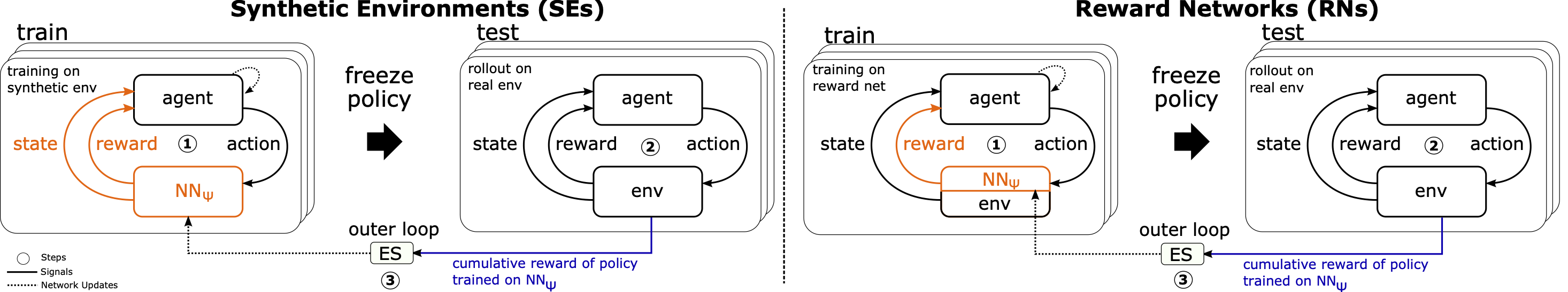We explore meta-learning agent-agnostic neural Synthetic Environments (SEs) and Reward Networks (RNs) for efficiently training Reinforcement Learning (RL) agents. While an SE acts as a full proxy to a target environment by learning about its state dynamics and rewards, an RN resembles a partial proxy that learns to augment or replace rewards. We use bi-level optimization to evolve SEs and RNs: the inner loop trains the RL agent, and the outer loop trains the parameters of the SE / RN via an evolution strategy. We evaluate these methods on a broad range of RL algorithms (Q-Learning, SARSA, DDQN, Dueling DDQN, TD3, PPO) and environments (CartPole and Acrobot for SEs, as well as Cliff Walking, CartPole, MountaincarContinuous and HalfCheetah for RNs). Additionally, we learn several variants of potential-based reward shaping functions. The learned proxies allow us to train agents significantly faster than when directly training them on the target environment while maintaining the original task performance. Our empirical results suggest that they achieve this by learning informed representations that bias the agents towards relevant states, making the learned representation surprisingly interpretable. Moreover, we find that these proxies are robust against hyperparameter variation and can also transfer to unseen agents.

Paper link: tba

Download Trained SE and RN Models

All SE and RN models can be downloaded here: https://www.dropbox.com/sh/fo32x0sd2ntu2vt/AACjv7RJ0CvfqwCXhTUZXqgwa?dl=0

Installation

Dependencies: python3, torch, gym, numpy, mujoco-py (only in case of learning RNs for HalfCheetah-v3 environment). We also use hpbandster for 1) three-level optimization with BOHB and 2) for parallel + distributed NES optimiziation, i.e. for job scheduling and communication between workers and masters in a distributed setting. Below scripts are for SLURM but can easily be adapted to any other job scheduling software.

The packages can be installed using the requirements.txt file:

pip install -r requirements.txt

Documentation

Optimizing Hyperparameters for Learning Synthetic Environments (initial three-level optimization with BOHB)

Overall structure

Several scripts in the experiments folder make use of the three-level optimization approach.

• outer loop: BOHB
• middle loop: NES (in scripts referred to as "GTN-RL")
• inner loop: RL

During parallelization, the logic is as follows: A single BOHB master orchestrates several BOHB workers (done by the BOHB package). Every BOHB worker corresponds to a NES master and every NES master (referred to as "GTN" -> see GTN_master.py) orchestrates several NES workers
(GTN_worker.py) via file IO. In each NES outer loop the NES master writes an individual input file and an input check file (the latter just prevents the first file from being read too early) to all of its NES works. After they finished calculations, they write a result file and a result check file, which is then read again by the NES master.

To ensure that the individual files can be distinguished, every NES master and worker can be uniquely identified by a combination of its BOHB-ID (assigned to the NES master and all NES workers of a single BOHB worker) and its ID (assigned individually to each NES worker). The general file types for file IO between NES master and NES workers thus are:

   
    _
    
     _input.pt 

     
      _
      
       _input_check.pt

       
        _
        
         _result.pt 
         
          _
          
           _result_check.pt 
          
         
        
       
      
     
    
   

Many scripts allow the BOHB-ID to be chosen manually whereas the ID for the different NES workers must span the range [0,X] with X as the number of NES workers per NES master.

Example

To start a BOHB script (in this example: experiments/GTNC_evaluate_cartpole_params.py) with two BOHB workers (i.e. two NES master) and 3 NES slaves per NES master, execute the following procedure:

• ensure that the values in the loaded config file (look up the .py file to see which yaml file is loaded) are set to proper values:

agents.gtn.num_workers: 3

• run the individual files in parallel. After setting the PYTHONPATH environment variable to the repository base folder, run in the command line:

python3 GTN_Worker.py 0 0 &
python3 GTN_Worker.py 0 1 &
python3 GTN_Worker.py 0 2 &
python3 GTN_Worker.py 1 0 &
python3 GTN_Worker.py 1 1 &
python3 GTN_Worker.py 1 2 &
python3 GTNC_evaluate_cartpole_params.py 0 3 &
python3 GTNC_evaluate_cartpole_params.py 1 3 &

An easier way on the slurm cluster would be the use of two scripts, the first script to call the NES workers (change absolute paths where necessary):

#!/bin/bash
#SBATCH -p bosch_cpu-cascadelake # partition (queue)
#SBATCH -t 3-23:59 # time (D-HH:MM)
#SBATCH -c 1 # number of cores
#SBATCH -a 0-5 # array size
#SBATCH -D /home/user/learning_environments # Change working_dir
#SBATCH -o /home/user/scripts/log/%x.%N.%A.%a.out # STDOUT  (the folder log has to exist) %A will be replaced by the SLURM_ARRAY_JOB_ID value, whilst %a will be replaced by the SLURM_ARRAY_TASK_ID
#SBATCH -e /home/user/scripts/log/%x.%N.%A.%a.err # STDERR  (the folder log has to exist) %A will be replaced by the SLURM_ARRAY_JOB_ID value, whilst %a will be replaced by the SLURM_ARRAY_TASK_ID

export LD_LIBRARY_PATH=/usr/local/cuda-9.0/lib64:$LD_LIBRARY_PATH
export LD_LIBRARY_PATH=/usr/local/cuda/lib64:$LD_LIBRARY_PATH
export LD_LIBRARY_PATH=/usr/local/cuda-10.0/lib64:$LD_LIBRARY_PATH

echo "source activate"
source ~/master_thesis/mtenv/bin/activate
echo "run script"
export PYTHONPATH=$PYTHONPATH:/home/user/learning_environments
export LD_LIBRARY_PATH=$LD_LIBRARY_PATH:/home/user/.mujoco/mjpro150/bin
bohb_id=$(($SLURM_ARRAY_TASK_ID/3+0))
id=$(($SLURM_ARRAY_TASK_ID%3))
cd experiments
python3 -u GTN_Worker.py $bohb_id $id
echo "done"

and the second script to call BOHB respectively the NES master (change absolute paths where necessary):

#!/bin/bash
#SBATCH -p bosch_cpu-cascadelake # partition (queue)
#SBATCH -t 3-23:59 # time (D-HH:MM)
#SBATCH -c 1 # number of cores
#SBATCH -a 0-2 # array size
#SBATCH -D /home/user/learning_environments # Change working_dir
#SBATCH -o /home/user/scripts/log/%x.%N.%A.%a.out # STDOUT  (the folder log has to exist) %A will be replaced by the SLURM_ARRAY_JOB_ID value, whilst %a will be replaced by the SLURM_ARRAY_TASK_ID
#SBATCH -e /home/user/master_thesis/scripts/log/%x.%N.%A.%a.err # STDERR  (the folder log has to exist) %A will be replaced by the SLURM_ARRAY_JOB_ID value, whilst %a will be replaced by the SLURM_ARRAY_TASK_ID

export LD_LIBRARY_PATH=/usr/local/cuda-9.0/lib64:$LD_LIBRARY_PATH
export LD_LIBRARY_PATH=/usr/local/cuda/lib64:$LD_LIBRARY_PATH
export LD_LIBRARY_PATH=/usr/local/cuda-10.0/lib64:$LD_LIBRARY_PATH

echo "source activate"
source ~/master_thesis/mtenv/bin/activate
echo "run script"
export PYTHONPATH=$PYTHONPATH:/home/user/learning_environments
export LD_LIBRARY_PATH=$LD_LIBRARY_PATH:/home/user/.mujoco/mjpro150/bin
cd experiments
bohb_id=$(($SLURM_ARRAY_TASK_ID+0))
python3 -u GTNC_evaluate_cartpole.py $bohb_id 3
echo "done"

A third alternative is to run everything (single NES master and multiple NES workers) on a single PC, e.g for debug purposes All the scripts in the experiments folder containing a "run_bohb_serial" method support this feature. Just call

python3 GTN_Worker_single_pc.py &
python3 GTNC_evaluate_cartpole_params.py &

Training Synthetic Environments after HPO

To train synthetic environments, run the corresponding "GTNC_evaluate_XXX.py" script, e.g.

GTNC_evaluate_gridworld.py
GTNC_evaluate_acrobot.py
GTNC_evaluate_cartpole.py

as described in the "Example" section before. It might be necessary to modify some parameters in the corresponding .yaml file. The trained synthetic environments are then called within other functions to generate the plots as described in the "Visualizations scripts" section

Training Reward Networks after HPO

To train reward environments, run the corresponding "GTNC_evaluate_XXX_reward_env.py" script if there exists a "GTNC_evaluate_XXX.py" script as well. In all other cases the script is called "GTNC_evaluate_XXX.py", e.g.

GTNC_evaluate_gridworld_reward_env.py
GTNC_evaluate_cartpole_reward_env.py
GTNC_evaluate_cmc.py
GTNC_evaluate_halfcheetah.py

The detailed procedure how to run these scripts is described in the "Example" section before. It might also be necessary to modify some parameters in the corresponding .yaml file. The only difference is that these scripts feature another input parameter specifying the "mode", i.e. type of used RL agent / reward environment:

• -1: ICM
• 0: native environment (no reward env)
• 1: potential function (exclusive)
• 2: potential function (additive)
• 3: potential function with additional info vector (exclusive)
• 4: potential function with additional info vector (additive)
• 5: non-potential function (exclusive)
• 6: non-potential function (additive)
• 7: non-potential function with additional info vector (exclusive)
• 8: non-potential function with additional info vector (additive)
• 101: weighted info vector as baseline (exclusive)
• 102: weighted info vector as baseline (additive)

The trained reward environments are then called within other functions to generate the plots as described in the "Visualizations scripts" section

Visualizations scripts

Please note that for the visualization scripts we assume existing trained SEs and RNs (see previous section how to train these or furhter above how to download them). Simply place the SEs and RNs in the corresponding directory. Below figure enumeration corresponds to paper figure enumeration.

Figure 2

Place the model directories Synthetic Environments/GTNC_evaluate_cartpole_2020-12-04-12 and Synthetic Environments/GTNC_evaluate_acrobot_2020-11-28-16 under results/. If you want to train the models from scratch, run GTNC_evaluate_cartpole.py with optimized parameters (default_config_cartpole_syn_env.yaml) and GTNC_evaluate_acrobot.py with optimized parameters (default_config_acrobot_syn_env.yaml) as described in the "Example" section. Then run

python3 experiments/GTNC_visualize_cartpole_acrobot_success_perc.py.py

with appropriate "LOG_DIRS" variable.

Figure 3 and 7

There are two variants to produce these figures:

1. run the evaluation on existing SE models from scratch (for generating the SE models, see above)
2. use the outputs of our evaluation.

Variant 1

Download the directories Synthetic Environments/GTNC_evaluate_cartpole_vary_hp_2020-11-17-10 and Synthetic Environments/GTNC_evaluate_acrobot_vary_hp_2020-12-12-13 and place them in results/. Now adjust the model_dir path inside experiments/syn_env_evaluate_cartpole_vary_hp_2.py or experiments/syn_env_evaluate_acrobot_vary_hp_2.py and run the script with the mode parameter (mode 0: real env, mode 1: syn. env. (no vary), mode 2: syn. env. (vary)) which correspond to the three different settings (train: syn/real HP: fixed/varying) of Figure 3 and 7. These scripts will produce the data for the DDQN curves and hereby create .pt files which can be processed for visualization (see variant 2) below). Repeat the process for the transfers for Dueling DDQN and discrete TD3 with the following files:

experiments/syn_env_evaluate_cartpole_vary_hp_2_DuelingDDQN.py
experiments/syn_env_evaluate_cartpole_vary_hp_2_TD3_discrete.py
experiments/syn_env_evaluate_acrobot_vary_hp_2_DuelingDDQN.py
experiments/syn_env_evaluate_acrobot_vary_hp_2_TD3_discrete.py

Now execute the steps in variant 2 below.

Variant 2

Download the directory Synthetic Environments/transfer_experiments (see link above) and move it to experiments/. Now run experiments/GTNC_visualize_cartpole_vary_hp_kde_plot.py for the density plot and experiments/GTNC_visualize_cartpole_vary_hp_barplot.py for the barplot (adjust the FILE_DIRS paths at the top of the file accordingly). For Acrobot (Figure 7) run experiments/GTNC_visualize_acrobot_vary_hp_kde_plot.py and experiments/GTNC_visualize_acrobot_vary_hp_barplot.py, respectively.

Figure 4 and 8

Download the directories Synthetic Environments/GTNC_evaluate_cartpole_vary_hp_2020-11-17-10 and Synthetic Environments/GTNC_evaluate_acrobot_vary_hp_2020-12-12-13 and place them in results/. Now adjust the dir path inside experiments/GTNC_visualize_cartpole_histogram.py or experiments/GTNC_visualize_acrobot_histogram.py and select the agentname you want to plot the histograms for.

Figure 5 and 9

There are two variants to produce these figures:

1. use directly the outputs of our evaluation.
2. run the evaluation on existing SE models from scratch (for generating the SE models, see above)

Variant 1

Download the directories

Reward Networks/evaluations/cartpole_compare_reward_envs
Reward Networks/evaluations/cliff_compare_reward_envs
Reward Networks/evaluations/cmc_compare_reward_envs
Reward Networks/evaluations/halfcheetah_compare_reward_envs

and place them in results/ (only the environment folders without the structure above). Now, run any of the following scripts:

python3 experiments/GTNC_visualize_gridworld_compare_reward_envs.py
python3 experiments/GTNC_visualize_cartpole_compare_reward_envs.py
python3 experiments/GTNC_visualize_cmc_compare_reward_envs.py
python3 experiments/GTNC_visualize_halfcheetah_compare_reward_envs.py

or any of the following scripts for varied hyperparameter plots:

python3 experiments/GTNC_visualize_gridworld_transfer_vary_hp.py
python3 experiments/GTNC_visualize_cartpole_transfer_vary_hp.py
python3 experiments/GTNC_visualize_cmc_transfer_vary_hp.py
python3 experiments/GTNC_visualize_halfcheetah_transfer_vary_hp.py

or any of the following scripts for transfer plots:

python3 experiments/GTNC_visualize_gridworld_transfer_vary_hp.py
python3 experiments/GTNC_visualize_cartpole_transfer_vary_hp.py
python3 experiments/GTNC_visualize_cmc_transfer_vary_hp.py
python3 experiments/GTNC_visualize_halfcheetah_transfer_vary_hp.py

Variant 2

To generate the content of

Reward Networks/evaluations/cartpole_compare_reward_envs
Reward Networks/evaluations/cliff_compare_reward_envs
Reward Networks/evaluations/cmc_compare_reward_envs
Reward Networks/evaluations/halfcheetah_compare_reward_envs

first download the directories (only the environment folders without the structure above)

Reward Networks/with reward threshold objective/Cliff
Reward Networks/with reward threshold objective/CartPole-v0
Reward Networks/with reward threshold objective/MountainCarContinuous-v0
Reward Networks/with reward threshold objective/HalfCheetah-v3

and place them in results/. Now run

python3 experiments/GTNC_evaluate_gridworld_compare_reward_envs.py 
   
    
python3 experiments/GTNC_evaluate_cartpole_compare_reward_envs.py 
    
     
python3 experiments/GTNC_evaluate_cmc_compare_reward_envs.py 
     
      
python3 experiments/GTNC_evaluate_halfcheetah_compare_reward_envs.py 
      

      
     
    
   

with appropriate LOG_DICT and SAVE_DIR variables and mode as additional script input as described in the "Training Reward Networks after HPO" section.

Do the same for varying hyperparameters experiments:

python3 experiments/GTNC_evaluate_x_transfer_vary_hp.py 
   

   

and the transfer experiments:

python3 experiments/GTNC_evaluate_x_transfer_algo_hp.py 
   

   

replace x with cartpole, gridworld, cmc or halfcheetah. Then follow the approach described in Variant 1 to produce the figures.

Figure 10

Download all subfolders in Reward Networks/with reward threshold objective/Cliff and place them in results/. Now run

python3 experiments/GTN_visualize_gridworld_learned_reward_env.py

and adjust the variable LOG_DIR at the top of the script with the approriate model with the suffix _1, _2, _5, or _6 which correspond o the RN types list in Section "Training Reward Networks after HPO" above (i.e. one sub-plot row of Figure 10). For each call of this script, there will be created one sub-plots of Figure 10 (simplified and non-simplified) and by turning on/off the SIMPLIFY flag you can choose whether to create the left or the right sub-plot.

Figure 11

Download the directory Synthetic Environments/GTNC_evaluate_step_size_2020-11-14-19and place it in results/. Now run

python3 experiments/GTNC_visualize_gridworld_step_size.py

with appropriate log_dir variable. For creating the directory yourself, run experiments/GTNC_evaluate_gridworld_step_size.py as described in the "Example" section above.

Supervised Learning / MBRL Baseline Experiment Results

Evaluation / results on five supervised models:

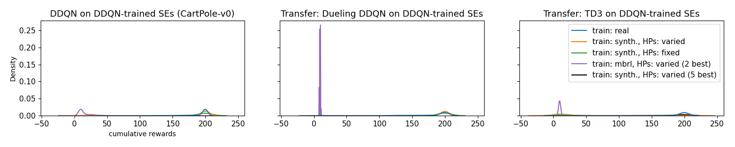
Comparing the cumulative test reward densities of agents trained on SEs (green and orange), supervised baseline (purple), and baseline on real environment (blue). Agents trained on the supervised model underperform the SE models and the real baseline.

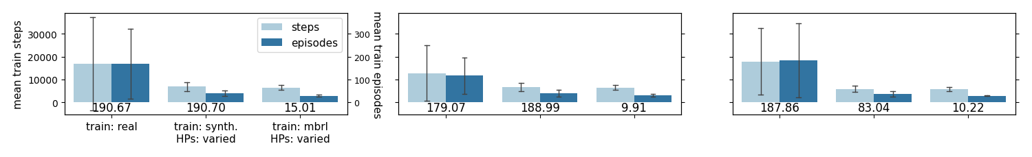Comparing the needed number of test steps and test episodes to achieve above cumulative rewards. Left: real baseline, center: SEs, right: supervised (mbrl) baseline

Evaluation / results on two of the best supervised models:

Comparing the cumulative test reward densities of agents trained on SEs (green and orange), supervised baseline (purple), and baseline on real environment (blue) using all five supervised models. Agents trained on the supervised model underperform the SE models and the real baseline and using only the best two supervised models does not seem to change this.

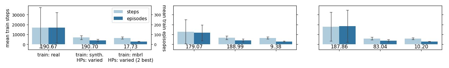Comparing the needed number of test steps and test episodes to achieve above cumulative rewards only using the best two of the five models. Left: real baseline, center: SEs, right: supervised (mbrl) baseline

Exemplary loss curve:

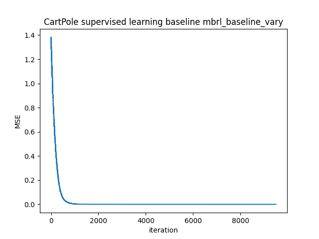
Across models, the MSE drops to ~5e-07 in the end.